3Affine algebraic curves
We will define an affine plane algebraic curve over a field as the zero set , where is an irreducible polynomial. So (at least in this chapter) we do not allow algebraic curves to have more than one component i.e., is not considered an algebraic curve.Algebraic curves are, in a sense we will not have time to explain, algebraic geometric objects of dimension one. The next step on the ladder is algebraic surfaces. Here we could consider , where . An example plot is given below, where and . This surface could be called the Valentine's surface.3.1 Intersection of two plane curves
Below you see an extract from Disquisitiones Arithmeticae of relevance in the proof of Lemma 3.2.
- and
- If and , then for .
If are polynomials with no common prime factors, then there exists
with
Let and .
If have no common factors in , they also have
no common factors in , which is a PID. Therefore
for suitable .
Multiplying by a suitable polynomial , we can clear the denominators on the left hand side
and get the result.
Get inspired by the proof of Lemma 3.2 and explain
how the extended euclidean algorithm applied to the polynomials
in (which is a euclidean ring!) helps in finding a polynomial , such that
Can we be sure that ?Macaulay2 code - viewer discretion advised
Use Lemma 3.2 to show that is a finite set, when
and have no common factors.
We consider two polynomials with no common prime factors.
As we saw in Lemma 3.2 this implies that
is finite. It could be empty. The distant goal is to prove that in the
right setting and intersect in preciselt
points.
Let be polynomials with no common factors,
and . Then
Let and . We let denote the
finite dimensional vector space of polynomials of degree .
in .
Check that
Define for ,
Notice that
for . This is because and
are relatively prime (no common factors). Now
consider the subspaces and
and use the isomorphism :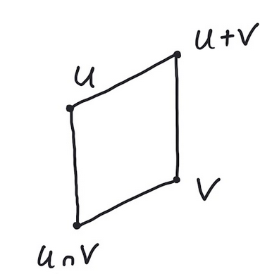 to conclude that
is equal to minus the dimension of or
, which is
Running this through a computer algebra system you magically end up with .Since we have a surjective homomorphism
it follows that .In fact, suppose that
are polynomials so that are linearly independent in . Choosing
, the equivalence classes
now in must be linearly independent,
because we cannot find
unless .
to conclude that
is equal to minus the dimension of or
, which is
Running this through a computer algebra system you magically end up with .Since we have a surjective homomorphism
it follows that .In fact, suppose that
are polynomials so that are linearly independent in . Choosing
, the equivalence classes
now in must be linearly independent,
because we cannot find
unless .
Below we generate two random cubics in two variables
over and output the dimenson (or rather degree of
) of .
The example given above are random cubics.
Find examples of and in the Macaulay2 window above so that the degree becomes strictly
less than .
Given a polynomial , there is a very natural way
of associating a homogeneous polynomial by
Suppose that , then
Similarly having a homogeneous polynomial
we can dehomogenize by
For ,
Notice here that
However,
Similar to the situation in , we can also
homogenize a polynomial and
obtain a homogeneous polynomial .
Explain how this is done.For an ideal , we define
i.e., as the ideal in generated by for
.Is it true that
Suppose that have no common factors and
that and do not intersect at infinity i.e.
Then
where and . Here we assume .
It is not too difficult to compute the points at infinity for a
polynomial. Write the highest degree terms in as . Here
is a homogeneous polynomial of degree and
survives in without any multiplication of a power of .
As is algebraically closed, we may write
for ,
since
for and
because is algebraically closed.The points at infinity of are
If and do not have any common points at infinity, then
and are relatively prime polynomials.This implies that
and therefore that
in the notation used in the proof of Proposition 3.5.Let us explain (3.3). Suppose that
Then with . Let us assume that
are picked so that is minimal. A moment of reflection will
convince you that
since we must have and .
As and are relatively prime, . Therefore there
exists a polynomial , such that
Now focus on
3.2 Rational functions and local rings
The quotient ring is an integral domain and we denote its field of fractions by . The elements in are called rational functions on .Notice that
A rational function is defined at if
there exists , such that
and . The pole set of is the set of points on , where
is not defined.
The pole set of is the zero set of the ideal , where
The pole set is finite. Also, if is defined at , then
its value is well defined by
where .
Observe that is a denominator for if and only if .If , then has to be a pole for . If not, then with
, but . If , we may find ,
such that and . Therefore is not a pole of .
We are assuming that is an irreducible polynomial. If and
, then . Therefore is finite by
Exercise 3.4.If with and , then
since . Therefore
Let . What is the value of the rational function
evaluated at ? What about ?
Suppose that is an arbitrary commutative ring with ideals . Then
the colon ideal is defined by
Suppose that you have a rational function . Then its pole set is the
zero set of the ideal from Proposition 3.13. If is
represented by , then
Here are some examples in Macaulay2 related to the computation of using
computation of the socalled colon ideal.
3.2.1 The local ring at a point
A local ring is a commutative ring with precisely one
maximal ideal.
Define
and the ring of power series
over .
- Prove that is a subring of and that they both are local rings. Show that
- Show that the field of fractions of is the Laurent series ring over .
- Show that is not an algebraically closed field.
- One can prove that is an algebraically closed field (Puiseux series) containing . Is algebraically closed if is an algebraically closed field of characteristic ?
Let . Then we let denote the subset of given by the rational
functions defined at . This is a subring of and contains as a subring:
Prove that is a local ring and that its unique maximal ideal
is formed by the rational functions with .
Suppose that . Show that the maximal ideal in is given
by i.e. it is the ideal
Prove that
3.3 Dimension in local rings
Consider , where is any field and and have no common factors in . Then we know by Proposition 3.5 that where and .We now wish to zoom in one of the finitely many points in . We do this by focusing on the local ringDefine the ideal
To get grounded, consider first the one variable case and for example
along with the point . Then
Show that and thatCheck that
where . , whereas .
Prove that if .
3.4 The crucial isomorphism
Suppose that with , where is algebraically closed. For each we have a well defined canonical homomorphism given by . Our objective is to show that is an isomorphism -algebras and therefore that3.4.1 Constructing orthogonal idempotents in
We are proving that is an isomorphism by constructing socalled orthogonal idempotents in i.e., elements satisfying for and . These correspond to the natural basis elements in the product ring on the right hand side of (3.5). A first approach is to work with polynomials , such that . We know these polynomials from the proof of Corollary 2.39.Does it work to put ? Certainly vanishes on , but this does not necessarily imply that . We only have . We need to adjust to make it work. This is done using Theorem 2.38 (the Hilbert Nullstellensatz).Notice that , where denotes the (maximal) ideal of polynomials vanishing on . For example, if . By Theorem 2.38, for sufficiently big . We keep this fixed for the rest of the proof.The elements that make (3.6) work are , where Notice that for a suitable polynomial by the binomial expansion of . Therefore for and for every . This implies that by Lemma 3.25. We continue to use this lemma below.Also if , then for every and finally So we see that and since it also belongs to for .3.4.2 Comaximal ideals
Is it true in general that
for ideals in a commutative ring ?
Two ideals in a commutative ring are called
comaximal if .
Suppose that and are comaximal ideals. Prove that and
that and are comaximal for every .
3.4.3 The image of the orthogonal idempotents
We have constructed orthogonal idempotents . They will do their magic when is applied to them. First, notice that is a unit in , since . This gives for . Finally this implies We realize the canonical basis vectors of the right hand side of (3.5) as images of . But we need more.3.4.4 Fractions are polynomials!
If and , then there exists , such that
, where .
Assume that and put . Then
where , so that . Therefore with . Notice that we have once again used Lemma 3.25.
The geometric series rules. It rules!
Notice that Lemma 3.30 actually says that
in (since ).
3.4.5 Injectivity
Suppose that and . This means that for every . Therefore there exists with and for . Now use the notation to conclude since for . We have used Lemma 3.30 times.3.4.6 Surjectivity
For a fraction we have (using Lemma 3.30) with for , that and therefore that in . We get . If presented with we see that where for .
Consider the two plane curves and in , where
Show that and do not intersect at . Now
zoom in on . What is
where ? Compare the dimension with
the output of