4Projective plane curves

We now move into projective territory, where we handle lines as points i.e., points will now be lines through zero in $K^3$ . Such points are elements of the projective plane $\mathbb{P}^2(K)$ over the field $K$ . In more precise terms

$\mathbb{P}^2(K) = \{[x, y, z] \mid (x, y, z)\in K^3\setminus\{0\}\},$ where $[x, y, z] = [\lambda x, \lambda y, \lambda z]$ for $\lambda\in K\setminus\{0\}$ .

We aim for Bezout's theorem (see Theorem 4.8), which is a small miracle. Think about it. We have two equations $f, g\in K[x, y]$ with no common solutions i.e., $V(f, g) = \emptyset$ . Then we homogenize them and suddenly $V(f^*, g^*) \neq \emptyset$ in $\mathbb{P}^2$ . Try to prove this from scratch!

4.1 Rational functions on the projective plane

It does not really make sense to view polynomials $K[x, y, z]$ as functions on $\mathbb{P}^2(K)$ . Not even homogeneous polynomials define functions in this setting. We can however study a very particular subfield

$K(\mathbb{P}^2) \subset K(x, y, z)$

given by

$k(\mathbb{P}^2) = \left\{\frac{A}{B}\, \middle|\, A, B \text{ homogeneous and } \deg(A) = \deg(B)\right\}.$

If $A/B\in k(\mathbb{P}^2)$ and $B(P) \neq 0$ , then $A(P)/B(P)$ is independent of the representative used for $P\in \mathbb{P}^2(K)$ . So, it actually makes sense to consider rational functions on $\mathbb{P}^2$ .

For $P\in \mathbb{P}^2$ may also define a local subring

$\mathcal{O}_P = \left\{r\in K(\mathbb{P}^2) \middle| r \text{ is defined at } P\right\} \subset K(\mathbb{P}^2).$

The map $\varphi: K(\mathbb{P}^2) \rightarrow K(x, y)$ given by

$\varphi\left(\frac{A}{B}\right) = \frac{A_*}{B_*}$ is an isomorphism of fields. If $P = [a, b, 1]$ , then

$\varphi(\mathcal{O}_P) = R_{(a, b)},$ where $R = K[x, y]$ .

Let $F, G\in K[x, y, z]$ be homogeneous polynomials. For $(F, G)\subset K[x, y, z]$ , we define the ideal $(F, G) \mathcal{O}_P \subset \mathcal{O}_P$ by

$\begin{aligned} (F, G) \mathcal{O}_P = \Bigg\{\frac{H_1 F + H_2 G}{B}\, \Bigg| \, & \deg(H_1 F) = \deg(H_2 G) = \deg(B),\\ & H_1, H_2, B \text{ are homogeneous polynomials in } K[x, y, z] \text{ with } B(P) \neq 0\Bigg\}. \end{aligned}$

If $P = [a, b, 1]$ , then for $\varphi$ defined in Exercise 4.1,

$\varphi((F, G) \mathcal{O}_P) = (F_*, G_*) R_{(a, b)},$ where $R = K[x, y]$ .

4.2 Homogeneous polynomials with no common factors

Let $F, G\in K[x, y, z]$ be homogeneous polynomials with no common factors. Then $V(F) \cap V(G) \subset \mathbb{P}^2$ is finite.

Recall the definition

$\mathbb{P}_z^2 = \{[a, b, c] \mid c \neq 0\}$ and similarly for $x$ and $y$ . It suffices to prove that $V(F) \cap V(G) \cap \mathbb{P}^2_z$ is finite and similarly for $x$ and $y$ . But

$V(F, G) \cap \mathbb{P}^2_z = V(F_*, G_*) \subset K^2$ and $F_*$ and $G_*$ have no common factors, since $F$ and $G$ had no common factors.

4.3 Projective transformations

An invertible matrix $T\in \operatorname{GL}_3(K)$ gives rise to a bijection $\mathbb{P}^2 \rightarrow \mathbb{P}^2$ . Also, $T$ induces an algebra isomorphism

$T^*: K[x, y, z] \rightarrow K[x, y, z]$ given by $T^*(f) = f\circ T^{-1}$ . In more brutal terms, if

$T^{-1} = \begin{pmatrix} a_{11} & a_{12} & a_{13}\\ a_{21} & a_{22} & a_{23}\\ a_{31} & a_{32} & a_{33} \end{pmatrix},$ then

$\begin{aligned} T^*(x) &= a_{11} x + a_{12} y + a_{13} z\\ T^*(y) &= a_{21} x + a_{22} y + a_{23} z\\ T^*(z) &= a_{31} x + a_{32} y + a_{33} z \end{aligned}$

If $F$ is a homogeneous polynomial, then $T^*(F)$ is also a homogeneous polynomial and

$T(V(F)) = V(T^*(F)) = V(F\circ T^{-1}).$

Consider $F = y$ and $G = x y - z^2$ . These two projective curves intersect at $[1, 0, 0]$ i.e., they intersect at $\infty$ , but their affine cousins $f = y$ and $x y - 1$ do not intersect. We can move $[1, 0, 0]$ to the "finite" affine plane, by using the projective transformation $T$ given by

$\begin{aligned} T([1, 0, 0]) &= [0, 0, 1]\\ T([0, 1, 0]) &= [0, 1, 0]\\ T([0, 0, 1]) &= [1, 0, 0]. \end{aligned}$ Then

$\begin{aligned} T^*(x) &= z\\ T^*(y) &= y\\ T^*(z) &= x \end{aligned}$ and

$T(V(F, G)) = V(y, y z - x^2).$ You see that $V(F, G)$ is transformed into a set of points with no points at $\infty$ (having $z = 0$ ).

4.4 Invariance under projective transformations

A projective transformation $T$ gives an isomorphism $T^*: K(\mathbb{P}^2) \rightarrow K(\mathbb{P}^2)$ , such that $\mathcal{O}_P$ maps isomorphically to $\mathcal{O}_{T(P)}$ and $(F, G)\mathcal{O}_P$ maps isomorphically to $(F\circ T^{-1}, G\circ T^{-1}) \mathcal{O}_{T(P)}$ .

$\dim_K \mathcal{O}_P/ (F, G) \mathcal{O}_P = \dim_K \mathcal{O}_{T(P)}/(F\circ T^{-1}, G\circ T^{-1}) \mathcal{O}_{T(P)}.$

4.5 Statement and proof of Bezout

Now we have reached the crown jewel of the course: Bezout's theorem. We have done must of the work in the previous chapter. We just need to move intersection points at $\infty$ into the finite affine plane in order to apply Proposition 3.11. Also $R/I$ from the left hand side of the arrow in (3.5) does not make sense in the projective case, but the right hand side of (3.5) does. Let us define the intersection multiplicity of the two plane projective curves $V(F)$ and $V(G)$ at $P\in \mathbb{P}^2(K)$ by

$I(P, F\cap G) = \dim_K \mathcal{O}_P/(F, G) \mathcal{O}_P.$

Let $F, G\in K[x, y, z]$ be homogeneous polynomials with no common components. Then

$\deg(F) \deg(G) = \sum_{P\in V(F) \cap V(G)} I(P, F\cap G).$

Suppose that

$V(F) \cap V(G) = \{P_1, \dots, P_r\}$ with

$\begin{aligned} P_1 &= [x_1, y_1, z_1]\\ &\vdots\\ P_r &= [x_r, y_r, z_r] \end{aligned}$ A line in $\mathbb{P}^2$ is a subset $L\subset \mathbb{P}^2$ of the form

$L = V( a x + b y + c z )$ with at least one of $a, b, c$ is non-zero. Why does there exist a line $L$ , such that

$P_1, \dots, P_r \not\in L?$

We assume the existence of such a line. Given $L$ , we may find a projective transformation $T$ , such that

$T(L) = V(z).$ It follows that $F' = F\circ T^{-1}$ and $G' = G\circ T^{-1}$ have no common points at the line at infinity $V(z)$ . Therefore we may assume that $V(F, G, z) = \emptyset$ . Since $F$ and $G$ have no common divisors, this implies (why?) that $z$ does not divide $F$ and $z$ does not divide $G$ .

But then $F_*$ and $G_*$ will have to have relatively prime highest degree components and therefore Proposition 3.11 applies to give the result (notice that $\deg(F_*) = \deg(F)$ and $\deg(G_*) = \deg(G)$ ).

4.6 Some more local algebra and local geometry

A discrete valuation ring (DVR) is a noetherian local domain $(R, \mathfrak{m})$ (not a field!),

where the maximal ideal $\mathfrak{m}$ is principal. A generator of $\mathfrak{m}$ is called a uniformizing parameter.

If $R$ is a DVR with uniformizing parameter $\pi\in R$ , then for every $r\in R$ , there exists a unique $n\in \mathbb{N}$ , such that

$r = u \pi^n,$ where $u$ is a unit in $R$ . The function $\nu: R\setminus\{0\}\rightarrow \mathbb{N}$ given by $\nu(r) = n$ is called a valuation ( $\pi$ -adic) and is independent of the choice of generator for the maximal ideal. It has the following properties

$\nu(r s) = \nu(r) + \nu(s)$ .
$\nu(r + s) \geq \min(\nu(r), \nu(s))$ .

Let $K$ be a field. Then the local ring

$K[x]_x = \left\{\frac{f(x)}{g(x)} \middle| x \nmid g(x)\right\} \subset K(x)$ is a DVR with maximal ideal $(x)$ . Similarly

$\mathbb{Z}_p = \left\{\frac{a}{b} \middle| p\nmid b\right\} \subset \mathbb{Q}$ is a DVR with maximal ideal $(p)$ , where $p$ is a prime number.

Suppose that $R$ is a DVR with maximal ideal $(\pi)$ and $R/(\pi) = K$ . Assume that $K \subset R$ , such that $R \rightarrow R/(\pi) = K$ splits. Prove that an element $r$ in $R/(\pi^n)$ has a unique expansion

$r = \lambda_0 + \lambda_1 \pi + \cdots + \lambda_{n-1} \pi^{n-1},$ where $\lambda_i\in K$ .

What is the connection to the local geometry of algebraic curves? For simplicity, let us fix the point $P = (0, 0)\in K^2$ consider $P\in V(F)$ . Then we may write

$F = F_m + F_{m+1} + \cdots, \tag{4.1}$ where $m \geq 1$ and $F_j$ is a form of degree $j$ . The lowest degree $F_m$ factors into a product of lines. These lines are called the tangent lines at $P$ .

You can experiment a bit with sage below to illustrate this.

The tangent lines of

$F = y^2 - x^2(x+1) = y^2 - x^2 - x^3 = (y+x)(y-x) - x^3$ are $y - x$ and $y + x$ .

The $m$ in (4.1) is called the multiplicity for $V(F)$ at $P$ . It is denoted $m_P(F)$ . If $m_P(F) = 1$ , we call $P$ a simple point on $V(F)$ .

How is the definition of mutliplicity generalized to an arbitrary point $P = (a, b)$ ?

Here is the (beautiful) connection to local algebra. Do not forget to look back at Definition 3.19.

Let $F\in K[x, y]$ be an irreducible polynomial. Then $P\in V(F)$ is a simple point if and only if the local ring $\mathcal{O}_P(F)$ is a DVR. Any line $L$ through $P$ , which is not the tangent line may be used as a uniformizing parameter $\pi = [L]\in \mathcal{O}_P(F)$ .

Let us just assume that $x$ is the tangent line at $P$ and $L = y$ . We know that $(x, y)\mathcal{O}_P(F)$ is the maximal ideal in $\mathcal{O}_P(F)$ . In the local ring at $P$ we have

$F = x u + g y,$ where $u$ is a unit. Therefore $x\in (y)$ . To prove the converse i.e., that $P$ is a simple point if $\mathcal{O}_P(F)$ is a DVR, we need Theorem 4.17.

Let $F\in K[x, y]$ be an irreducible polynomial and let $\mathfrak{m}$ denote the maximal ideal in $\mathcal{O}_P(F)$ . Then

$m_P(F) = \dim_K \mathfrak{m}^n/\mathfrak{m}^{n+1}$ for $n\gg 0$ .

Let $\mathfrak{m}$ denote the maximal ideal in $\mathcal{O}_P(F)$ and $I= (x, y)\subset K[x, y]$ . Notice that $\mathfrak{m} = I \mathcal{O}_P(F)$ . Using the exact sequence (see Fulton, page 28 for more on exact sequences of modules)

$0\rightarrow \mathfrak{m}^n/\mathfrak{m}^{n+1} \rightarrow \mathcal{O}_P(F)/\mathfrak{m}^{n+1} \rightarrow \mathcal{O}_P(F)/\mathfrak{m}^n\rightarrow 0$ of vector spaces, it suffices to show that $\dim_K \mathcal{O}_P(F)/\mathfrak{m}^n = n\, m_P(F) + s$ for a constant $s$ for $n \gg 0$ . Assume that $P = (0, 0)$ . From our crucial result in Section 3.4, we know that

$K[x, y]/(I^n, F) \cong \mathcal{O}_P/(I^n, F)\mathcal{O}_P \cong \mathcal{O}_P(F)/I^n \mathcal{O}_P(F) = \mathcal{O}_P(F)/\mathfrak{m}^n,$ where $\mathcal{O}_P$ is the local ring of rational functions on $K^2$ defined at $P$ . For $n \geq m = m_P(F)$ consider the exact sequence

$0 \rightarrow K[x,y]/I^{n-m} \xrightarrow{F} K[x, y]/I^n \rightarrow K[x, y]/(I^n, F) \rightarrow 0,$ while quietly recalling that $\dim_K K[x, y]/I^n = n(n+1)/2$ .

Given polynomials $f, g\in R = K[x, y]$ and a point $P\in K^2$ , show that the natural homomorphism

$R_P \rightarrow \left(R/(f)\right)_P\Big/ g \left(R/(f)\right)_P = \Gamma(f)_P\Big/ [g] \Gamma(f)_P = \mathcal{O}_P(f)\Big/ [g] \mathcal{O}_P(f)$ is surjective with kernel $(f, g) R_P$ .

Finally we have the following result.

Let $P$ be a simple point on $V(F)$ . Suppose that $G\in K[x, y]$ . Then

$I(P, G\cap F) = \nu([G])$ in $\mathcal{O}_P(F)$ . Here $\nu$ denotes the valuation in the DVR $\mathcal{O}_P(F)$ .

Here we make use of the isomorphism (see Exercise 4.18)

$\mathcal{O}_P/(G, F) \mathcal{O}_P \rightarrow \mathcal{O}_P(F) / G \mathcal{O}_P(F)$ and Exercise 4.12.

4.7 Max Noether's theorem

Max Noether was the father of Emmy Noether. He worked extensively on algebraic geometry and we shall present one of his results. First some notation.

Let $F$ and $G$ denote two projective algebraic curves with no common components and $P\in \mathbb{P}^2$ . Then we define

$I(P, F\cap G) = \dim_K \mathcal{O}_P/(F, G)\mathcal{O}_P$ and the intersection cycle

$F\cdot G = \sum_{P\in V(F, G)} I(P, F\cap G) P.$

Suppose that $H\cdot F \geq G\cdot F$ (it is almost clear what this means, right?). Noether's theorem addresses the existence of a projective algebraic curve $B$ , such that

$B\cdot F = H\cdot F - G\cdot F. \tag{4.2}$

Such a $B$ may be found provided that $H = A F + B G$ i.e., $H\in (F, G)$ , since then

$(A F + B G)\cdot F = BG \cdot F = B\cdot F + G \cdot F. \tag{4.3}$

We have used in (4.3) that we have an exact sequence

$0 \rightarrow \mathcal{O}_P/(B, F) \xrightarrow{\cdot G} \mathcal{O}_P/(G B, F) \rightarrow \mathcal{O}_P/(G, F) \rightarrow 0$ of vector spaces over $K$ : $I(P, (G B) \cap F) = I(P, G\cap F) + I(P, B\cap F)$ .

When is $H = A F + G B$ satisfied? The following (local to global) result due to Noether clarifies this.

$H\in (F, G) \iff H \in (F, G)\mathcal{O}_P$ for every $P\in V(F, G)$ .

We will only prove the local to global direction. We may assume that $V(F, G, z) = \emptyset$ . From the affine case (section 3.4), we conclude that $H_* = a F_* + b G_*$ and therefore that $Z^m H = A F + B G$ for some $m\gg 0$ . But since the multiplication map

$K[x, y, z]/(F, G) \xrightarrow{Z} k[x, y, z]/(F, G) \tag{4.4}$ is injective, we get $H\in (F, G)$ . Well, let us see why multiplication by $Z$ is injective in (4.4). It is actually a nice proof: for a general homogeneous polynomial $J\in k[x, y, z]$ , we let $J_0 = J(x, y, 0)\in k[x, y]$ . Suppose that $z H = A F + B G$ . Then $A_0 F_0 + B_0 G_0 = 0$ . Since $V(F, G, z) = \emptyset$ , $A_0 = \lambda G_0$ and $B_0 = \mu F_0$ and

$z H = (A - \lambda G) F + (B + \lambda F) G$ and we see that $z\mid A-\lambda G$ and $z\mid B + \lambda F$ , since $(A - \lambda G)_0 = 0$ and $(B + \lambda G)_0 = (B - \mu G)_0 = 0$ .

When $P$ is a simple point on $F$ and $I(P, H\cap F) \geq I(P, G\cap F)$ , then $H_*\in (F, G)\mathcal{O}_P$ .

We have $\nu(H) \geq \nu(G)$ in $\mathcal{O}_P(F)$ by Lemma 4.19. Therefore $H_*\in (G_*)\subset \mathcal{O}_P(F)$ . As $\mathcal{O}_P(F_*)/(G_*) \cong \mathcal{O}_P/(F_*, G_*)$ by Exercise 4.18, we get that $H_*\in (F_*, G_*)$ at $P$ .

4.8 Elliptic curves

Elliptic curves are simply plane projective curves of degree three with only simple points i.e., non-singular cubics. They are among the most surprising and beautiful objects in all of modern mathematics. This is mainly due to the fact that they carry an abelian group structure.

Let $C$ be an irreducible cubic and $C', C''$ cubics. Suppose that

$C'\cdot C = P_1 + \cdots + P_8 + P_9, \tag{4.5}$ where $P_1, \dots, P_9$ are simple points on $C$ , and suppose that $C''\cdot C = P_1 + \cdots + P_8 + Q$ . Then $Q = P_9$ .

Suppose that $Q\neq P_9$ . Let $L$ be a line through $P_9$ not passing through $Q$ with

$L\cdot C = P_9 + R + S.$ Then

$(L C'')\cdot C = C'\cdot C + Q + R + S. \tag{4.6}$ Comparing (4.5) with (4.6) we may, using Lemma 4.23, find a line $L'$ , such that

$L'\cdot C = Q + R + S.$ But we must have $L = L'$ .

4.8.1 Addition on an elliptic curve

Let $C$ be an elliptic curve i.e., $C = V(F)$ , where $F$ is homogeneous of degree three with only simple points. For two points $P, Q\in C$ we define $\varphi(P, Q) = R$ , where

$L \cdot C = P + Q + R.$ Of course this gives a commutative operation, but we need a neutral element $\mathcal{O}\in C$ . Now we define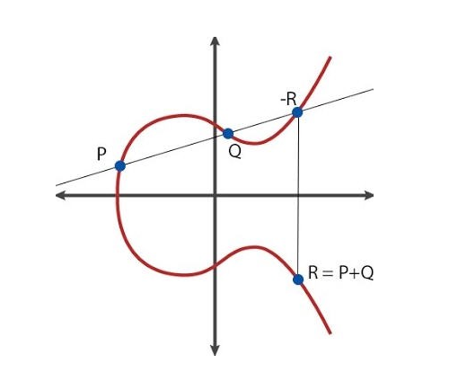

$P\oplus Q = \varphi(\mathcal{O}, \varphi(P, Q)).$

The operation $\oplus$ makes $C$ into an abelian group.

We only need to check that $\oplus$ is associative i.e.,

$\varphi(\varphi(\mathcal{O}, \varphi(P, Q)), R) = \varphi(\varphi(\mathcal{O}, \varphi(R, Q)), P).$ We list the intersection cycles and end up with a good idea. Here goes $(P\oplus Q) \oplus R$ :

$\begin{aligned} C\cdot PQ &= P + Q + P'\\ C\cdot \mathcal{O} P' &= \mathcal{O} + P' + S\\ C\cdot RS &= R + S + R' \end{aligned}$

Here is $P\oplus (Q \oplus R)$ :

$\begin{aligned} C\cdot QR &= Q + R + Q'\\ C\cdot \mathcal{O} Q' &= \mathcal{O} + Q' + T\\ C\cdot PT &= P + T + T' \end{aligned}$

The endgame is to prove $R' = T'$ . The magnificent trick appears now in using Proposition 4.24 for

$\begin{aligned} C' &= PQ \cdot RS \cdot \mathcal{O} Q'\\ C'' &= \mathcal{O} P' \cdot QR \cdot PT \end{aligned}$

4.8.2 Explicit formulas

Suppose that we have an elliptic curve $C = V(F)$ given by the affine equationOne may prove that, such an equation really defines an elliptic curve if the discriminant of the cubic polynomial on the right hand side is $\neq 0$ . Here the discriminant is

$a^2 b^2 - 4 b^3 - 4 a^3 c - 27 c^2 + 18 a b c.$

$y^2 = x^3 + a x^2 + b x + c$ with $\mathcal{O} = (0, 1, 0)$ .

Suppose that $f(x, y) = y^2 - P(x)$ , where $P\in k[x]$ is a polynomial of degree three. Prove that the corresponding projective plane cubic curve $V(f^*)$ has only simple points if and only if the discriminant of $P(x)$ is $\neq 0$ .

If $P_1 = (x_1, y_1)$ and $P_2 = (x_2, y_2)$ , how do we actually compute $P_3 = (x_3, y_3) = P_1\oplus P_2$ ?

First, we notice that $\mathcal{O}, (x_0, y_0, 1), (x_0, -y_0, 1)\in C$ all lie on the line $V(x - x_0 z)$ , so that $- P = (x_0, -y_0, 1)$ if $P = (x_0, y_0, 1)\in C$ .

If $x_1\neq x_2$ in $P_1$ and $P_2$ above, we consider the line $y = \alpha x + \beta$ through $P_1$ and $P_2$ . To find $x_3$ , we simply use the identity

$x^3 + a x^2 + b x + c - (\alpha x + \beta)^2 = (x - x_1) (x - x_2) (x - x_3). \tag{4.7}$ Comparing coefficients, this gives

$a - \alpha^2 = - (x_1 + x_2 + x_3)$ and therefore

$x_3 = \alpha^2 - a - x_1 - x_2. \tag{4.8}$ Of course here you already know that $\alpha = (y_2 - y_1)/(x_1 - x_2)$ .

What if $x_1 = x_2$ ? Well, if $P = P_1 = P_2$ , then we need to compute the tangent line at $P = (x_1, y_1)$ , which is

$\frac{\partial F}{\partial x}(x_1, y_1) (x - x_1) + \frac{\partial F}{\partial y}(x_1, y_1)(y-y_1) = (3 x_1^2 + 2 a x_1 + b)(x-x_1) + 2 y_1(y - y_1)$ Here our line is given by $\alpha = -(3 x_1^2 + 2 a x_1 + b)/(2 y_1)$ in (4.7) and we have a formula for the $x$ -coordinate in $2 P_1$ using (4.8).

Computing the $y$ -coordinate in both sums can be done by first finding the intersection of the relevant line with the $y$ -axis:

$\beta = y_1 - \alpha x_1.$ Then $y_3 = \alpha x_3 + \beta$ Woooops! This is wrong. In fact the right formula is

$y_3 = - \alpha x_3 - \beta.$ Why?

4.8.3 Machine computation in Sage

The computer algebra system Sage was originally built for experimenting with mathematics related to elliptic curves. Here is how to define the elliptic curve $y^2 = x^3 + a x + b$ over $\mathbb{Q}$ and compute with addition of points.

4.9 Fun and surprising facts

The following result is deep and non-trivial.

Let $E$ be an elliptic curve defined by a polynomial with coefficients in $\mathbb{Q}$ . Then $E(\mathbb{Q})$ is a finitely generated abelian group.

A finitely generated abelian group $A$ is isomorphic to a $A_{\operatorname{free}} \oplus A_{\operatorname{tors}}$ , where $A_{\operatorname{free}}$ is finitely generated free isomorphic to $\mathbb{Z}^r$ and $A_{\operatorname{tors}}$ is the finite torsion subgroup. The rank of $E(\mathbb{Q})$ is the dimension of $E(\mathbb{Q})_{\operatorname{free}}$ i.e., $r$ in $\mathbb{Z}^r$ .

For an elliptic curve $E$ as above, there are only finitely many possibilities for the torsion subgroup of $E(\mathbb{Q})$ . See Mazur's theorem. For some reason $E(\mathbb{Q})$ has no points of order $11$ and no points of order $>12$ . The points of finite order are available from the Nagell-Lutz theorem.

It is not known if the rank of $E(\mathbb{Q})$ is bounded, where $E$ runs through the elliptic curves over $\mathbb{Q}$ ! The current record for the rank is given by the Elkies curve

$\begin{aligned} &y^2 + x y + y = x^3 - x^2 -\\ &20067762415575526585033208209338542750930230312178956502 x + \\ &34481611795030556467032985690390720374855944359319180361266008296291939448732243429, \end{aligned}$ which has rank at least $28$ . The rank and the torsion subgroup can be computed for a given elliptic curve in Sage as illustrated below.