5Euclidean vector spaces
Big data are made up of many numbers in data sets. Such data sets can be represented as vectors in a high dimensional euclidean vector space. A vector is nothing but a list of numbers, but we need to talk mathematically about the size of a vector and perform operations on vectors. The term euclidean refers to vectors with a dot product as known from the plane .The purpose of this chapter is to set the stage for this, especially by introducing the dot product (or inner product) for general vectors. Having a dot product is immensely useful and we give several applications like linear regression and the perceptron learning algorithmIn the last part of the chapter rudimentary basics of analysis are introduced like sequences, continuous functions, open, closed and compact subsets. Some results will in this context only be quoted and not proved.5.1 Vectors in the plane
The dot product (or inner product) between two vectors is given by where We may also interpret and as matrices (or column vectors). Then the dot product in (5.1) may be realized as the matrix product: The length or norm of the vector is given by This follows from the Pythagorean theorem:
5.2 Higher dimensions
The notions of dot product, norm and the formula for cosine of the angle generalize immediately to vectors in dimensions higher than two.We denote the set of column vectors with rows by and call it the euclidean vector space of dimension . An element is called a vector and it has the form (column vector with entries) A vector in is a model for a data set in real life. A collection of numbers, which could signify measurements. You will see an example of this below, where a vector represents a data set counting words in a string.Being column vectors, vectors in can be added and multiplied by numbers: The dot product generalizes as follows to higher dimensions.5.2.1 Dot product and norm
The dot product of
is defined by
The norm of is defined by
A vector with is called a unit vector.Two vectors are called orthogonal if . We write
this as .
Show that
where .
Use the definition in (5.3) to show that
for and .
Let be a nonzero vector and . Use the definition
in (5.4) to show that
and that
is a unit vector.
You could perhaps use Exercise 5.3 to do this. Notice also that
is the absolute value for if .
Given two vectors with , find , such
that and are orthogonal, i.e.
 In this case, if is the angle between and , show that
Use this to show that
Finally show that
where and are two angles.
In this case, if is the angle between and , show that
Use this to show that
Finally show that
where and are two angles.
This is an equation, where is unknown!
For , it is sketched below
that if and are orthogonal, then
and are the sides in a right triangle.
In the last question, you could use that the vectors
are unit vectors.
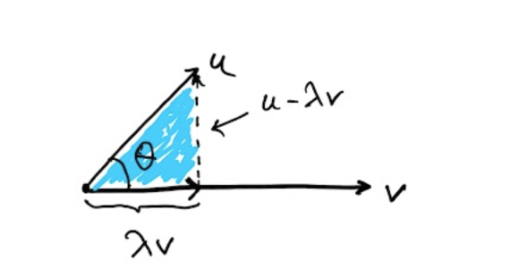
Given two vectors , solve the minimization problem
First convince yourself that minimizes
if and only if it minimizes
which happens to be a quadratic polynomial in .
Let denote the distance from to the line through and . What is true about ?
5.2.2 The dist formula from high school
The infamous dist formula from high school says that the distance from the point to the line given by is Where does this magical formula come from? Consider a general line in parametrized form (see Definition 4.9) If , then the distance from to is given by the solution to the optimization problem This looks scary, but simply boils down to finding the top of a parabola. The solution is and the point on closest to is .Now we put (see Example 4.10) in order to derive (5.5). The solution to (5.6) becomes We must compute the distance from to in this case. The distance squared is This is a mouthful and I have to admit that I used symbolic software (see below) to verify that5.2.3 The perceptron algorithm
Already at this point we have the necessary definitions for explaining the perceptron algorithm. This is one of the early algorithms of machine learning. It aims at finding a high dimensional line (hyperplane) that separates data organized in two clusters. In terms of the dot product, the core of the algorithm is described below.A line in the plane is given by an equation for , where . Given finitely many points each with a label of (or blue and red for that matter), we wish to find a line (given by ), such that if (above the line) and if (below the line). In some cases this is impossible (an example is illustrated below).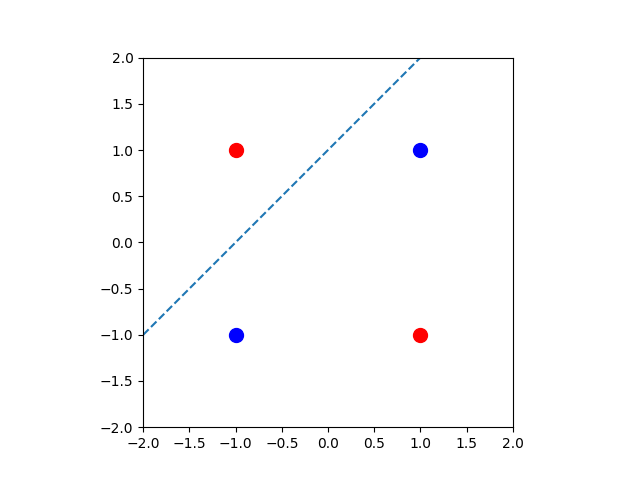
Given finitely many vectors , can we find
, such that
for every ?
Come up with a simple example, where this problem is unsolvable i.e., come
up with vectors , where such an does not
exist.Hint
In case exists, the following
ridiculously simple algorithm works in computing . It is called the perceptron (learning) algorithm.
Try out some simple examples for and .
- Begin by putting .
- If there exists with , then replace by and repeat this step. Otherwise is the desired output vector.
Let us try out the algorithm on the simple example of just
two points in given by
In this case the algorithm proceeds as pictured below.It patiently crawls its way ending with the vector , which
satisfies and .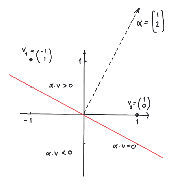
Let us see how (5.7) works in a concrete example.
Consider the points
in , where and are labeled by and is labeled by . Then we let
Now we run the simple algorithm above Example 5.9:
From the last vector we see that determines
a line separating the labeled points.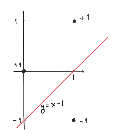
Consider the points
in , where the first point is labeled with and the rest by .
Use the perceptron algorithm to compute a separating hyperplane.What happens when you run the perceptron algorithm on the above
points, but where the label of
is changed from to ?
Why does the perceptron algorithm work?
We will assume that there exists , such that for every . This is equivalent to the existence of , such that for every .
Suppose that there exists , such that
for every . Show then that
there exists , such that
for every .
The basic insight
is the following
Let . Show that
works.
Let .
After iterations of the perceptron algorithm,
These statements follow from the inequalities
and
Proposition 5.13 implies that
Therefore we get and there is an upper bound on the number of
iterations used in the second step. At a certain iteration within this bound
we must have for every .
Below is an implementation of the perceptron (learning) algorithm
in python (with numpy) with input from Example 5.10 (it also works in higher dimensions).
5.2.4 Pythagoras and the least squares method
The result below is a generalization of the theorem of Pythagoras about right triangles to higher dimensions.
If and , then
This follows from
since .
The dot product and the norm have a vast number of applications. One of them is the
method of least squares: suppose that you are presented with a system
of linear equations, where is an matrix.You may not be able to solve (5.8). There could be for example
equations and only unknowns making it impossible for all the equations to hold.
As an example, the system
of three linear equations and two unknowns does not have any solutions.The method of (linear) least squares seeks the best approximate solution to (5.8) as a
solution to the minimization problemThere is a surprising way of finding optimal solutions to (5.10):
Suppose we know that is orthogonal to for every . Then
for every
by Proposition 5.14. So, in the case that
for every we have
for every proving that is an optimal solution to
(5.10).Now we wish to show that is orthogonal to for every if and
only if . This is a computation involving the matrix arithmetic
introduced in Chapter 3:
for every if and only if . But
so that .On the other hand, if for every , then for
every : if we could find with , then
for a small number . This follows, since
which is
By picking sufficiently small,
In a future course on linear algebra you will see that the system of linear equations in
Theorem 5.15 is always solvable i.e., an optimal solution to (5.10) can
always be found in this way.Mentimeter
Show that (5.9) has no solutions. Compute the best approximate solution to (5.9)
using Theorem 5.15.
The classical application of the least squares method is to find
the best line through a given set of points
in the plane .Usually we cannot find a line matching the points precisely. This corresponds to the fact that
the system of equations
has no solutions.Working with the least squares solution, we try to compute the best
line in the sense that
is minimized.
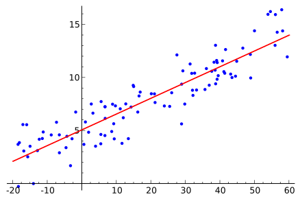
Best fit of line to random points from Wikipedia.
We might as well have asked for the best quadratic polynomial
passing through the points
in .The same method gives us the system
of linear equations.
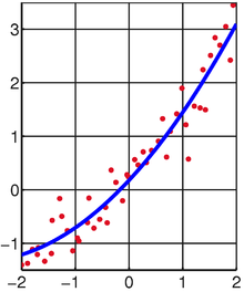
Best fit of quadratic polynomial to random points from Wikipedia.
The method generalizes naturally to finding the best polynomial of degree
through a given set of points.
Find the best line through the points
and and the best quadratic polynomial
through the points
and .It is important here, that you write down the relevant system
of linear equations according to Theorem 5.15.
It is however ok to solve the equations
on a computer (or check your best fit on WolframAlpha).Also, you can get a graphical illustration of your result in the sage window below.
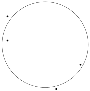
A circle with center and radius is given by the equation
- Explain how (5.12) can be rewritten to the equation where .
- Explain how fitting a circle to the points in the least squares context using (5.13) leads to the system of linear equations.
- Compute the best circle through the points
by giving the center coordinates and radius with two decimals. Use the Sage window
below to plot your result too see if it matches the drawing.
5.2.5 The Cauchy-Schwarz inequality
Even though the generalizations of the dot product and norm to higher dimensions amount to just adding some coordinates, they entail a rather stunning result called the Cauchy-Schwarz inequality. The proof is not long, but revolves around a rather beautiful trick.
For two vectors ,
We consider the function given by
Then is a quadratic polynomial with . Therefore
its discriminant must be i.e.,
which gives the result.
The Cauchy-Schwarz inequality
implies that
for two vectors and it makes sense to define the angle
between these vectors by
For arbitrary two numbers ,
since
Why is
for arbitary numbers ?
When vectors are interpreted as data sets,
the number in (5.14) is known as the cosine similarity
and measures the correlation between the two data sets
and .An application could be the similarity between two strings.
Consider the two strings
"Mathematics is fun and matrices are useful"
and
"Mathematics is fun and matrices are applicable".From the words in the two strings we form the following vectors in .where every word in the two strings has an entry counting the number of
occurences in the string. A measure for the equality between
the two strings is the cosine of the angle between the two vectors.The closer the cosine gets to (corresponding to an angle of
degrees), the more similar we consider the strings.In the above case the cosine similarity is approximately .Below is a snippet of python code (using numpy) for computing the cosine similarity of two strings, where
words are separated by blanks. It can be extended in many ways.
This application is based on rather basic mathematics, but we do get a quantitative measure for
how close two strings are. This is a crude tool applicable for flagging potential plagiarism.The cosine similarity is crucial in machine learning, especially in NLP.
On a more advanced (and modern!) level, we have the word embeddings. These are
maps from a finite set of words
to a potentially very high dimensional euclidean space . One usually
requires that two words and similar in meaning should have
close to in . A breakthrough occured in 2013, when Google
introduced the word embedding word2vec.
5.2.6 Distance of vectors and the triangle inequality
We know how to measure the size of a vector by its norm . We need to measure how close two vectors are i.e., we need to measure their distance. A perfectly good measure for the distance from to is the norm You can see from (5.4) that is small implies that the coordinates of and are close. Also we want if their distance is zero. This is satisfied. Similarly we want the distance from to to equal the distance from to . This is true, since for any vector .
Show the above, that for any vector . Explain why
this implies for every .
One other, not so obvious property, is the triangle inequality.
For two vectors ,
From the Cauchy-Schwarz inequality (Theorem 5.22) it follows that
Since the right hand side of this inequality is , the result follows.
Why is this result called the triangle inequality? A consequence is that
i.e., that the distance from to is always less than or equal to
the distance from to plus the distance from to , where
is a third vector.In boiled down terms: the length of any one side in a triangle is
less than or equal to the sum of the lengths of the two other sides.
Find two typos in the figure above. Correct them!
The triangle inequality implies that
for every .5.2.7 Bounded subsets
A subset is called bounded if there exists a (potentially very, very big) number , such that for every . Putting this is the same asThis condition is true if and only if (the norm is bounded)
Every finite subset is bounded (why?). For , (5.17) simply says
This implies that an interval is bounded by putting in (5.17).
Describe geometrically what it means for a subset of resp.
to be bounded by using intervals resp. circles (disks).
Show precisely that the subset of is not bounded, whereas the subset
is.
Sketch why
is bounded. Now use Fourier-Motzkin elimination to show the same
without sketching.
5.3 An important remark about the real numbers
In the beginning of this course, we postulated the existence of the real numbers as an extension of the rational numbers with their ordering .The rational numbers had the glaring defect that the graph of the function given by does not intersect the -axis between and in spite of the fact that and .It seems from the sage plot below, that the graph intersects the -axis around , but it really does not happen! Your computer and its screen only handles rational numbers.Surely the most natural property for a well behaved function (like ) is that it must intersect the -axis in a point with if and .I will not be completely precise about how to repair this defect about the rational numbers , but just state one exceedingly important property about the real numbers in the button below.In fact this one property guarantees that does not have any holes as in the graph above.Supremum and infimum5.3.1 Supremum
A subset of is called bounded from above if there exists , such that for every . Here is called an upper bound for .
Give an example of a subset of the real numbers, which is not bounded from
above and one that is.
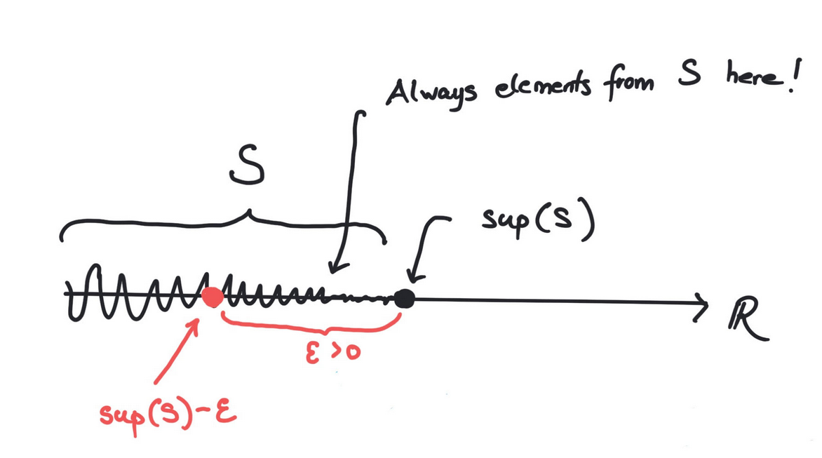
The set of real numbers satisfies that for every subset bounded from above,
there exists a smallest upper bound denoted called
the supremum of . In precise terms,
- for every
- If we move a little to the left of we encounter elements from : for every , there exists , such that
5.3.2 Infimum
In the same way a subset of is called bounded from below, if there exists , such that for every . Every subset bounded from below has a largest lower bound denoted called the infimum of . In precise terms,- for every
- If we move a little to the right of we encounter elements from : for every , there exists , such that
Give a simple example of a subset bounded from above, where
.Show that the subset of is bounded from above and below and
that and .
Show that is infinite if .
5.4 Sequences and limits in
For the first time in the notes we are now moving towards infinite processes. We will introduce limits of vectors organized in an infinite sequence.
A sequence
in is an infinite list of vectors
in , where repetitions are allowed. Such a sequence is denoted .
Below we give two examples of sequences in .
The first sequence is given by and the second for . The first sequence
explodes to infinity, whereas the second sequence gets closer and closer to . In the latter case we
write
What does it mean that a sequence of vectors in has limit ? Intuitively,
we can get as close to as we want by choosing
sufficiently big. Here is the precise way of saying this:If a sequence has a limit , then we write
A sequence is called convergent if it has a limit. Let us see
how our new technology works on two intuitively
obvious examples.
Let us use (5.18) to give a precise proof of
where . So given any we must find , such that
for . But
So we simply choose to be the smallest natural number bigger than .An even simpler example is a constant sequence like
i.e., for all . Here we want the limit to be and
(5.18) agrees. We can put :
If a sequence is convergent, then it can have
only one limit. You can not have a convergent sequence with two different limits!
In particular, the constant sequence
cannot converge to .
Give a precise proof of the fact that a convergent sequence can only have
one limit using proof by contradiction i.e., start by assuming that
it has two different limits . Then show that
cannot be true by showing that
Now, that we have the definition of a convergent sequence, we go on to use it in a rather
typical proof of a rather typical result. In this (typical) proof we first handle the
infinite and then the finite.
Try in the definition of being a limit and apply (5.15) to
A convergent sequence is bounded i.e., there exists , such that
for every .
Let denote the limit of . Then for , we may find
, such that for . Therefore
for by (5.15). Let
and then letting
, we see that
for every .
Proposition 5.39 shows that the sequence
cannot be convergent. Why?
What is the limit of the sequence
It does not have a limit.
Try to prove first that the sequence cannot converge to , by assuming that it does.
Let and be convergent sequences in with limits
and respectively. Then
- the sequence is convergent with limit .
- the sequence is convergent with limit (if )
- the sequence is convergent with limit provided that and for every (if ).
I will give the proof of (ⅱ.). By definition (see
(5.18)) we are given and we must find
, such that
for . An old trick shows that
Therefore we may find so that
where and for every (see Proposition 5.39).
We are assuming the and are convergent sequences. Therefore we may find
and in , so that
Choosing , we get
for .
The proof of (ⅰ.) in Proposition 5.42 is much less involved
than the given proof of (ⅱ.) in the same result. In the proof of
(ⅱ.) we used a trick using . Use the same
trick with and the triangle inequality to prove
(ⅰ.).
What is the limit of the sequence given by
It does not have a limit
Consider the sequence given by
Carry out a computer experiment in Sage below to find the limit
of . Can you prove what you observe in
the experiment?
Assume that is a convergent sequence in . Show that
is a convergent sequence in .
Let be a sequence bounded below with the property that
Show that is the limit of .Similarly let be a sequence bounded above with the property that
Show that is the limit of .
- Show that for .
- Prove that and for .
- Start with two numbers and with and define where and . Carry out computer experiments in the sage (python) window below to analyze the sequences and for different values of and .
- Prove for that if .
- Let and . Show that the limits exist and that .
5.4.1 Closed and open subsets
We have defined what it means for a subset of a euclidean space to be bounded. Now we come to an exceedingly important definition about subsets being closed meaning that they should (in a mathematically precise way) contain their boundary points. For example, we want the interval to be closed, whereas the interval should not be closed, because it is missing its boundary point .
A subset is called closed if it contains all its limit vectors. This
means that if is a convergent sequence contained in , then its limit must
be contained in .
The following subsets
are closed subsets of for every .
Let be finitely many closed subsets of . Then
are closed subsets of .
A subset is called open if is closed.
Prove that
are open subsets if are open subsets.
Let for , where .
Show that is an open subset of .
In fact, an arbitrary (also infinite) intersection of closed subsets is closed and an arbitrary (also infinite) union of open subsets is open. However, for a
first course introducing intersections and unions over arbitrary families is pushing the
envelope.
Infinite series5.4.2 Infinite series
Given a sequence in we may form the new sequence given by the sums Such a sequence is called an infinite series. It is denoted and is defined to converge if the sequence converges.Infinite series give rise to very beautiful identities like We will not go deeper into the rich theory of infinite series, but settle at defining a widely used infinite series called the geometric series. Let with . We saw in the first chapter that for any number . If , then .
Show that if .
Therefore
The series in (5.19) is called the geometric series.
Compute the (infinite) sums
The series given by i.e.,
is called the harmonic series. Explore the growth of the harmonic series as a function of
using the sage window below.What does this video
on twitter have to do with the harmonic series?Suppose that the inequality
holds. What does (5.20) imply for the harmonic series? Is (5.20) true? Compare
with the graphs in the sage window below.Use the sage window below to investigate if the sequence given by
converges. In particular, make a clever statement about the convergence by studying a finite table
of
observing for .
5.5 Continuous functions
A function , where and is
called continuous at if for every
convergent sequence in with limit , is a
convergent sequence with limit in . The function is called continuous
if it is continuous at every .
Let in Definition 5.59. We consider the two functions
where i.e., is the identity function and is a
constant function given by the real number . Both of these
functions are continuous. Let us see why.A sequence is convergent with limit if
according to (5.18). To verify Definition 5.59, we must prove that
But , so that the above claim is true
by (5.22) with the same .
Similarly . Here we may pick , since
to begin with.
We give now three important results, which can be used
in concrete situations to verify that a given function is continuous. They can
be proved without too much hassle. The first result below basically follows from the
definition of the norm of a vector (see (5.4)).
The functions given by
for are continuous. In general a function
is continuous if and only if
is continuous for every , where and
.
Suppose that and are continuous
functions, where and . Then
the composition
is continuous.
Let be functions defined on a subset . If
and are continuous, then the functions
are continuous functions, where (the last function is
defined only if ).
This result is a consequence of the definition of continuity and Proposition 5.42.
Show in detail that the function given by
is continuous by using Proposition 5.63 combined with
Lemma 5.61.
Verify the claim in Remark 5.65.
More advanced (transcendental) functions like and also turn out to be continuous.We are now in position to prove a famous result from 1817 due to Bolzano.
Let be a continuous function, where . If
and , then there exists with , such
that .
This is proved using the supremum property of the real numbers. The subset
is non-empty (since ) and bounded from above. We let .We will need the following observation about the continuous function :
If for , then there exists a small
, such that
for every .Similarly if for , then there exists a small
, such that
for every .These observations imply that by the definition
of supremum. Similarly we cannot according to these
observations have or .
In this case and by definition of supremum we have for every . But for some there must exist , such that .This is impossible.The only possibility remaining is .
Again, by Proposition 5.63, polynomials are continuous functions.
Now, as promised previously, we state and prove the following result.
Let
be a polynomial of odd degree, i.e. is odd. Then has a root,
i.e. there exists , such that .
We will assume that (if not, just multiply by ). Consider written as
By choosing negative with extremely big, we have ,
since is negative and
as is positive. Notice here that the terms
are extremely small, when is extremely big.Similarly by choosing
positive and tremendously big, we have .
By Theorem 5.67, there exists with with
.
Before defining (and more importantly giving examples of) closed subsets, we will
define abstractly the preimage of a subset of a function.
Consider a
function
where and are sets. If , then the
preimage of under is defined by
Consider the function , where and
given by
For , as illustrated below.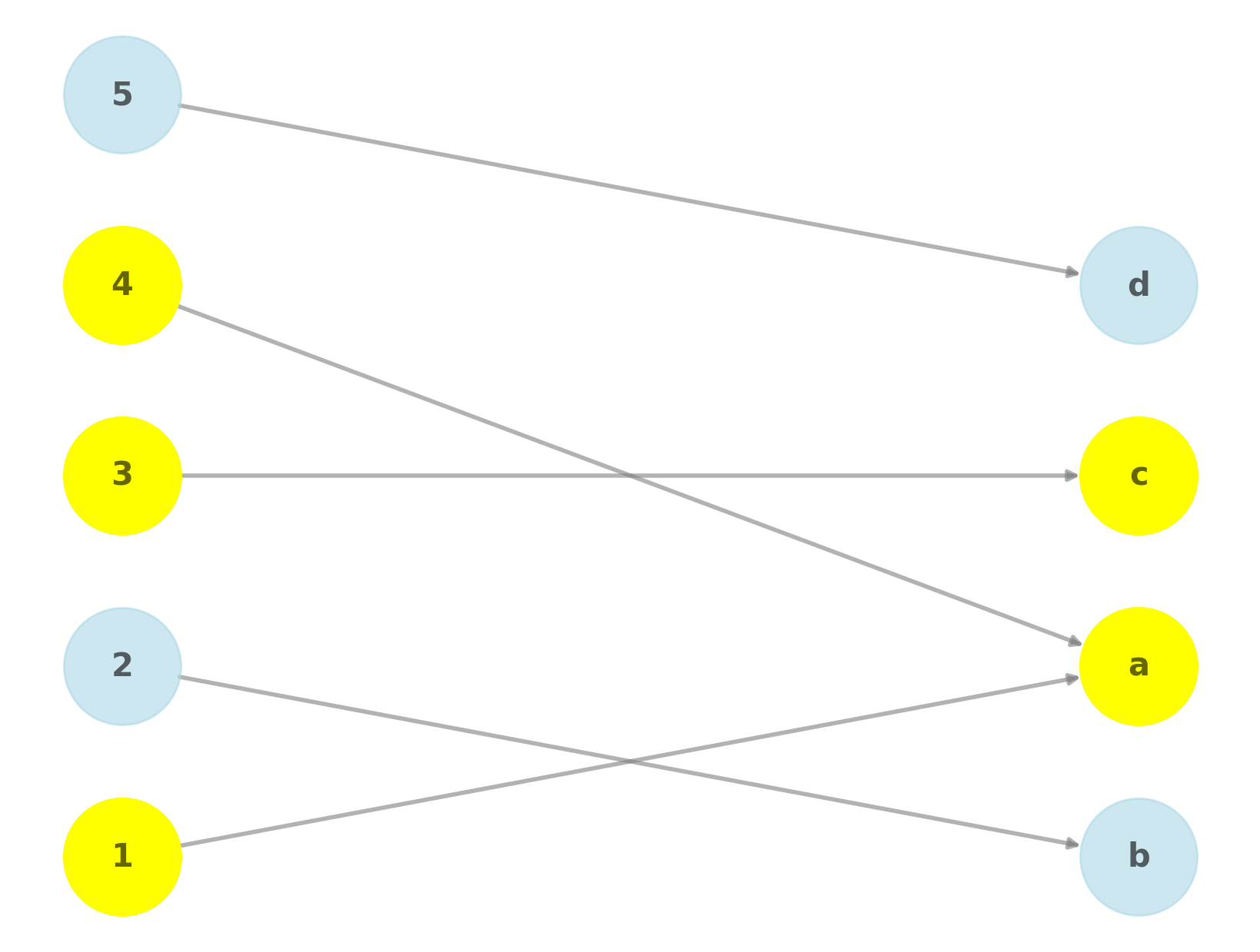
What is when and
?
Consider the function given by
and let . What is true about ?
If is a closed subset and
a continuous function, then the preimage
is a closed subset of .
Given a convergent sequence with and , we must prove that
by Definition 5.49. Since is continuous, it follows by Definition 5.59 that
. As is closed, we must have . Therefore by
Definition 5.69.
The function given by is
continuous. Therefore the subset
of is closed, since is a closed subset
of by Proposition 5.50.
Show thatis a continuous function , where and andUse Proposition 5.50 and Proposition 5.73 to show thatis a closed subset of .Hint
We end the section on continuous functions by introducing compact subsets
and a crucial optimization result.
Write
where is a suitable (closed) interval.
Experiment a bit and compute , when is close to . Is close to a special value when is close to ? What happens when is close to ? How do you explain this in terms of and ?
A subset of euclidean space is called compact if it is bounded and closed.
Let be a compact subset of and
a continuous function. Then there exists , such that
for every .